Lesson 3 Manipulate: tidyr, dplyr
Data scientists, according to interviews and expert estimates, spend from 50 percent to 80 percent of their time mired in the mundane labor of collecting and preparing data, before it can be explored for useful information. - NYTimes (2014)
Today we’re going to learn about a package by Hadley Wickham called dplyr and how it will help you with simple data exploration, and how you can use it in combination with the %>% operator for more complex wrangling (including a lot of the things you would use for loops for.
And we’re going to do this in Rmarkdown in the my-project repository we created this morning.
Here are the steps:
- Open RStudio
- Make sure you’re in your
my-projectrepo (and if not, get there) - New > Rmarkdown… (defaults are fine)
- Save as
gapminder-dplyr.rmd - Our workflow together will be to write some description of our analysis in Markdown for humans to read, and we will write all of our R code in the ‘chunks’. Get ready for the awesomeness, here we go…
Today’s materials are again borrowing from some excellent sources, including
- Dr. Jenny Bryan’s lectures from STAT545 at UBC: Introduction to dplyr
- Software Carpentry’s R for reproducible scientific analysis materials: Dataframe manipulation with dplyr
3.1 install our first package: dplyr
Packages are bundles of functions, along with help pages and other goodies that make them easier for others to use, (ie. vignettes).
So far we’ve been using packages included in ‘base R’; they are ‘out-of-the-box’ functions. You can also install packages from online. The most traditional is CRAN, the Comprehensive R Archive Network. This is where you went to download R originally, and will go again to look for updates.
You don’t need to go to CRAN’s website to install packages, we can do it from within R with the command install.packages("package-name-in-quotes").
## from CRAN:
#install.packages("dplyr") ## do this once only to install the package on your computer.

library(dplyr) ## do this every time you restart R and need it
select <- dplyr::select # overwrite raster::select
What’s the difference between install.packages() and library()? Here’s my analogy:
install.packages()is setting up electricity for your house. Just need to do this once (let’s ignore monthly bills).library()is turning on the lights. You only turn them on when you need them, otherwise it wouldn’t be efficient. And when you quit R, and come back, you’ll have to turn them on again withlibrary(), but you already have your electricity set up.
3.2 Use dplyr::filter() to subset data row-wise.
First let’s read in the gapminder data.
# install.packages('gapminder') # instead of reading in the csv
library(gapminder) # this is the package name
str(gapminder) # and it's also the data.frame name, just like yesterday
## Classes 'tbl_df', 'tbl' and 'data.frame': 1704 obs. of 6 variables:
## $ country : Factor w/ 142 levels "Afghanistan",..: 1 1 1 1 1 1 1 1 1 1 ...
## $ continent: Factor w/ 5 levels "Africa","Americas",..: 3 3 3 3 3 3 3 3 3 3 ...
## $ year : int 1952 1957 1962 1967 1972 1977 1982 1987 1992 1997 ...
## $ lifeExp : num 28.8 30.3 32 34 36.1 ...
## $ pop : int 8425333 9240934 10267083 11537966 13079460 14880372 12881816 13867957 16317921 22227415 ...
## $ gdpPercap: num 779 821 853 836 740 ...filter() takes logical expressions and returns the rows for which all are TRUE. Visually, we are doing this (thanks RStudio for your cheatsheet):

filter(gapminder, lifeExp < 29)
filter(gapminder, country == "Rwanda")
filter(gapminder, country %in% c("Rwanda", "Afghanistan"))
Compare with some base R code to accomplish the same things
3.3 Meet the new pipe operator
Before we go any further, we should exploit the new pipe operator that dplyr imports from the magrittr package by Stefan Bache. This is going to change your data analytical life. You no longer need to enact multi-operation commands by nesting them inside each other. This new syntax leads to code that is much easier to write and to read.
Here’s what it looks like: %>%. The RStudio keyboard shortcut: Ctrl + Shift + M (Windows), Cmd + Shift + M (Mac).
Let’s demo then I’ll explain:
This is equivalent to head(gapminder). This pipe operator takes the thing on the left-hand-side and pipes it into the function call on the right-hand-side – literally, drops it in as the first argument.
Never fear, you can still specify other arguments to this function! To see the first 3 rows of Gapminder, we could say head(gapminder, 3) or this:
I’ve advised you to think “gets” whenever you see the assignment operator, <-. Similary, you should think “then” whenever you see the pipe operator, %>%.
You are probably not impressed yet, but the magic will soon happen.
3.4 Use dplyr::select() to subset the data on variables or columns.
Back to dplyr …
Use select() to subset the data on variables or columns. Visually, we are doing this (thanks RStudio for your cheatsheet):

Here’s a conventional call:
But using what we just learned, with a pipe, we can do this:
Let’s write it again but using multiple lines so it’s nicer to read. And let’s add a second pipe operator to pipe through head:
## # A tibble: 4 x 2
##    year lifeExp
##   <int>   <dbl>
## 1  1952    28.8
## 2  1957    30.3
## 3  1962    32.0
## 4  1967    34.0
Think: “Take gapminder, then select the variables year and lifeExp, then show the first 4 rows.”
3.5 Revel in the convenience
Let’s do a little analysis where we calculate the mean gdp for Cambodia.
Here’s the gapminder data for Cambodia, but only certain variables:
gapminder %>%
  filter(country == "Cambodia") %>%
  # select(country, year, pop, gdpPercap) ## entering 4 of the 6 columns is tedious
  select(-continent, -lifeExp) # you can use - to deselect columns
and what a typical base R call would look like:
## # A tibble: 12 x 4
##    country   year      pop gdpPercap
##    <fct>    <int>    <int>     <dbl>
##  1 Cambodia  1952  4693836      368.
##  2 Cambodia  1957  5322536      434.
##  3 Cambodia  1962  6083619      497.
##  4 Cambodia  1967  6960067      523.
##  5 Cambodia  1972  7450606      422.
##  6 Cambodia  1977  6978607      525.
##  7 Cambodia  1982  7272485      624.
##  8 Cambodia  1987  8371791      684.
##  9 Cambodia  1992 10150094      682.
## 10 Cambodia  1997 11782962      734.
## 11 Cambodia  2002 12926707      896.
## 12 Cambodia  2007 14131858     1714.
or, possibly?, a nicer look using base R’s subset() function:
## # A tibble: 12 x 4
##    country   year      pop gdpPercap
##    <fct>    <int>    <int>     <dbl>
##  1 Cambodia  1952  4693836      368.
##  2 Cambodia  1957  5322536      434.
##  3 Cambodia  1962  6083619      497.
##  4 Cambodia  1967  6960067      523.
##  5 Cambodia  1972  7450606      422.
##  6 Cambodia  1977  6978607      525.
##  7 Cambodia  1982  7272485      624.
##  8 Cambodia  1987  8371791      684.
##  9 Cambodia  1992 10150094      682.
## 10 Cambodia  1997 11782962      734.
## 11 Cambodia  2002 12926707      896.
## 12 Cambodia  2007 14131858     1714.
3.6 Use mutate() to add new variables
Imagine we wanted to recover each country’s GDP. After all, the Gapminder data has a variable for population and GDP per capita. Let’s add a new column and multiply them together.
Visually, we are doing this (thanks RStudio for your cheatsheet):

Exercise: how would you add that to the previous
filterandselectcommands we did with Cambodia:
Answer:
3.7 group_by and summarize
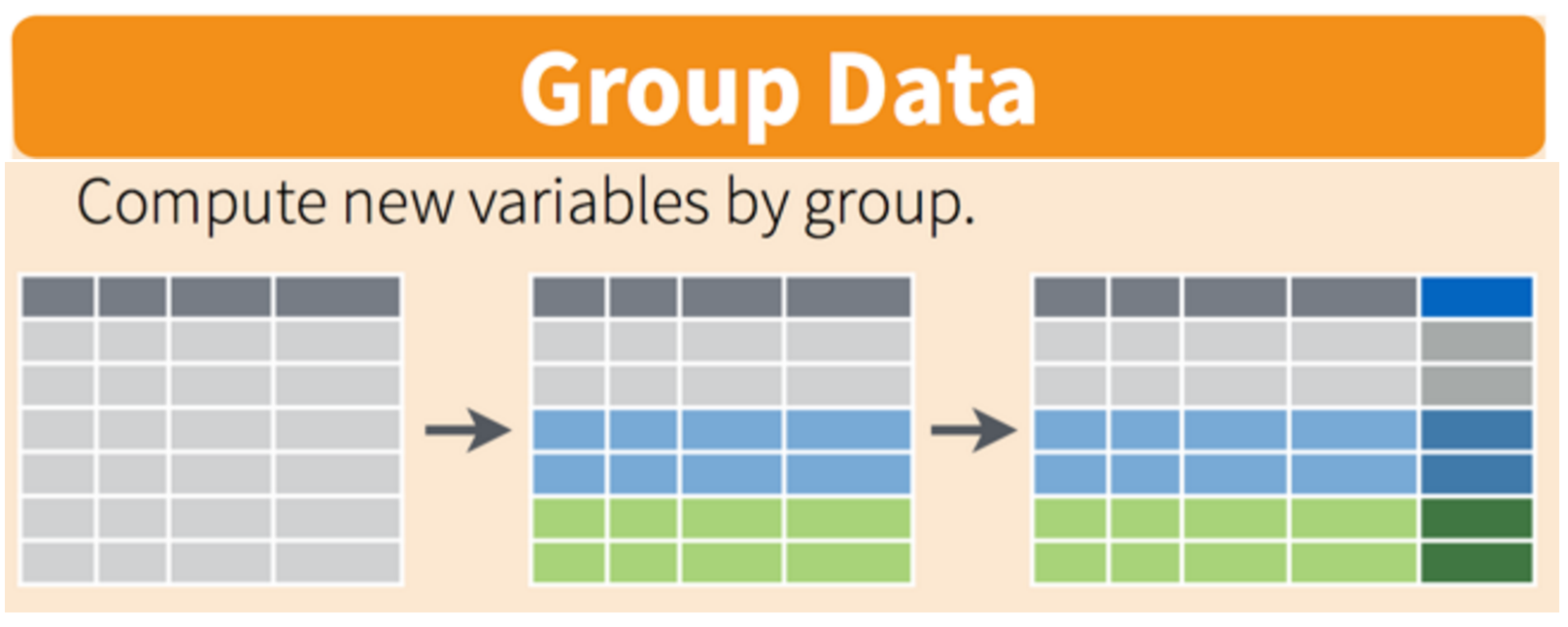
Great! And now we want to calculate the mean gdp across all years (Let’s pretend that’s a good idea statistically)
Visually, we are doing this (thanks RStudio for your cheatsheet):

3.8 Remember our for loop?
And how would you then do this for every country, not just Cambodia? Well, yesterday we would have been thinking about putting this whole analysis inside a for loop, replacing “Cambodia” with a new name each time we iterated through the loop. But today, we have it already, just need to delete one line from our analysis–we don’t need to filter out Cambodia anymore!!
Visually, we are doing this (thanks RStudio for your cheatsheet):

gapminder %>%
  select(-continent, -lifeExp) %>%
  mutate(gdp = pop * gdpPercap) %>%
  group_by(country) %>%
  summarize(mean_gdp = mean(gdp)) %>%
  ungroup() # if you use group_by, also use ungroup() to save heartache later
So we have done a pretty incredible amount of work in a few lines. Our whole analysis is this. Imagine the possibilities from here.
3.9 Summary
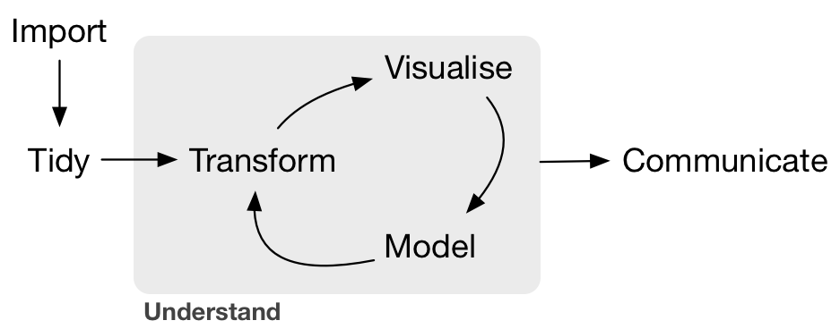
This has been the ‘Tranform’ or Wrangling part of this cycle.

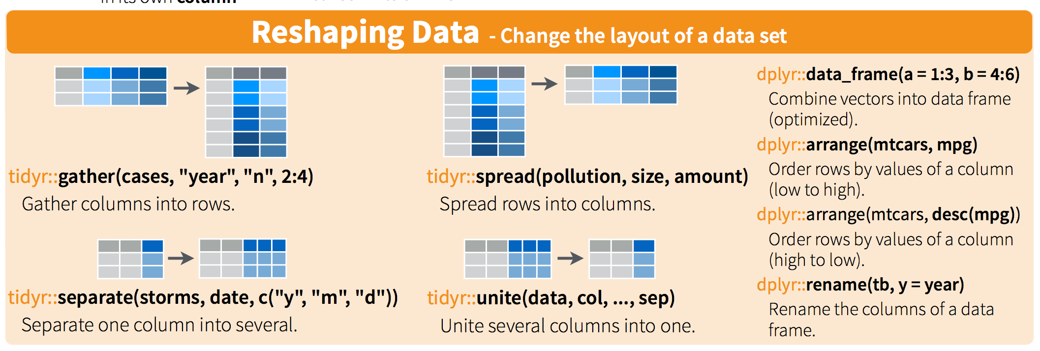
Importing and tidying is also a HUGE part of this process, and we don’t have time to get into it today. But look at the cheatsheet, and watch the webinar. cheatsheet and webinar. Watch this 1 hour webinar and follow along in RStudio and your science will be forever changed. Again!

3.10 Further materials as reference…
3.10.1 Rationale
When performing data analysis in R, code can become quite messy, making it hard to revisit and determine the sequence of operations. Commenting helps. Good variable names help. Still, at least two common issues make code difficult to understand: multiple variables and nested functions. Let’s examine these issues by approaching an analysis presenting both problems, and finally see how dplyr offers an elegant alternative.
For example, let’s ask of the surveys.csv dataset: How many observations of a certain thing you’re interested in appear each year?
3.10.2 Pseudocode
You can write the logic out as pseudocode which can become later comments for the actual code:
3.10.3 Summary
The tidyr and dplyr packages were created by Hadley Wickham of ggplot2 fame. The “gg” in ggplot2 stands for the “grammar of graphics”. Hadley similarly considers the functionality of the two packages dplyr and tidyr to provide the “grammar of data manipulation”.
Next, we’ll explore the data wrangling lessons that Remi contributed to Software Carpentry.